Facts around Structured Notes Usage - Advisor's perspective survey

US SEC registered market is about 45-60 bn in size. Internationally this market is much bigger owing to matured market in Europe and active investor demand in Asia and Latin America. These products are becoming important risk management tools in investor’s portfolios. They provide access to variety of markets where ETF’s or other products cannot reach by providing partial to full protection to capital. Despite these virtues, market participants complain about their complexity, illiquidity and transparency.
Recently Exceed Investments found after surveying 700 financial advisors that structural inefficiencies like, Illiquidity and transparency are holding back the latent demand for structured investors. “Exceed Investments is a New York-based financial services firm developing next-generation structured investments. The firm commissioned a third party to conduct studies on structured investment perceptions in both 2013 and 2014, culminating in the proprietary 2014 Exceed Structured Investments Report. The goal of the research was to identify overall advisor views on and usage of structured products, with an eye towards identifying which steps the industry can take to increase utilization and acceptance.”
Research methodology • Research leadership – WealthManagement.com, a Penton Media company • Participants – 707 completed advisor surveys • Participant selection – Members of the Wealthmanagement.com database; random selection • Motivation – Participation led to eligibility in a lottery for several American Express gift cards
Why do we use structured notes?
Today investing world is replete with variety of investment options including derivative products. Commonly asked question is if I need exposure to a particular asset I can invest in that asset directly by buying a stock, or mutual fund or an ETF. Even I can create such a product sometimes using Options on those assets. All of these are true to certain extent. But like the name structured notes provide customized risk and reward profiles.
For instance, Yesterday I was discussing with a friend of mine about a Reverse Convetible note issued by a large bank is good investment or not. He immediately fired back, what is the return on the note. I told him 6% per annum for 6 years in this low interest environment. Compare this to US Treasuries that offer mere 2%. Next question came to me what is my risk. To this I said, if the index underlying Reverse Convertible goes below 50% of the initial index level on the maturity date you will lose corresponding capital otherwise you will get full return of capital. Now this kind of note can be deployed by understanding the Risk/reward metrics both historically and in probable future scenarios.
Below survey of Advisors speaks exactly to this fact that people want to use structured notes by understanding the Risk and Reward of these products.

Next question comes to mind is okay, you need structured notes but what features are most desirable. During my same discussion about the structured investments yesterday, another friend told me people are afraid of repeat of 2008 scenario. That is they want protection from secular decline in the market. This has been captured clearly by the Exceed investments survey on desirable features below. Most of the investors are looking for capital protection.

Alright, we know now some of the motivations behind the need for a structured investment. Then are these products being used more often or less often? Not surprisingly they are being use less as per survey below and my informal conversations. Most investors who lost their money investing in these products have considered moving away from them and some other have not understood these products so they do not have any interest.

We see in this chart, that structured notes are being used in very small portions despite their benefits. I guess this is so because of limited information about these products.

Now that we have looked at why structured notes are preferred and still not part of the overall portfolios. Let us take a look at some drivers for avoiding these products. Below survey speaks loud and clear these products are too complicated to understand and they tend to be highly illiquid. On the point of being too complicated I agree to some extent only. I agree products with strange names like Air Bag auto callable, Trigger phoenix autocallables, high low range accrual etc might confound an ordinary investor. I would think for an investor who is adept at handling latest mobile phone gadgets and navigating through them in 21st century spending some time to understand these products is time well spent. On the point of illiquidity, I think more people start holding these products market will start building its own secondary market.

I am a strong advocate of transparency around, the information on the structured note issuance, their market values and understanding of the underlying derivatives. Now as more and more people start understanding these products and associated risks and rewards we think market will improve. As you are witnessing in the Over the Counter derivatives markets, after moving the transactions to Swap exchange facilities and cleared space we are seeing spreads becoming narrower. This is natural consequence of the opening up markets. One important thing I found interesting in the survey is to reduce the minimum size. Now many issuers are currently coming up with products with small unit sizes.

Another important facet in the structured note business is distribution channel. Most of the distribution is being conducted via Wirehouses

If you are provided access to these structured products so that you can possibly help your investing clients benefit from these products. Most of them are still in the state of confusion rather than jump onto investing in the structured notes. This clearly indicates, Access to markets, understanding of the markets are both required to fully realize benefits of this market I am actively advocating for transparency in the structured note markets through products like, Structured note database to what is on the market, Independent pricing to discover the market values and training and education to understand these markets better.

Structured Note Issuance summary June 1-13-2014

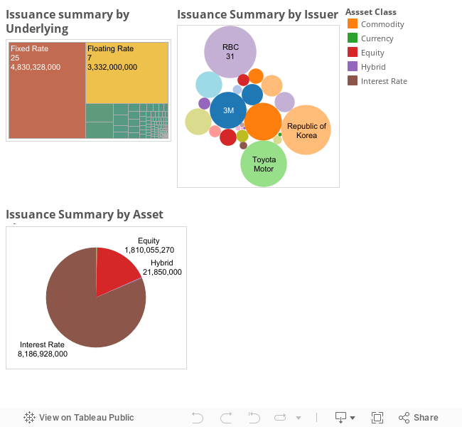
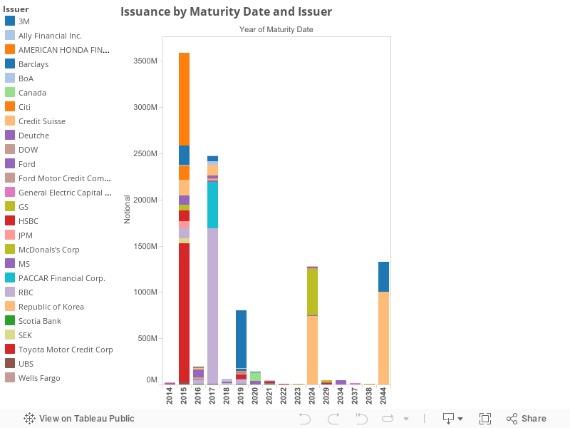
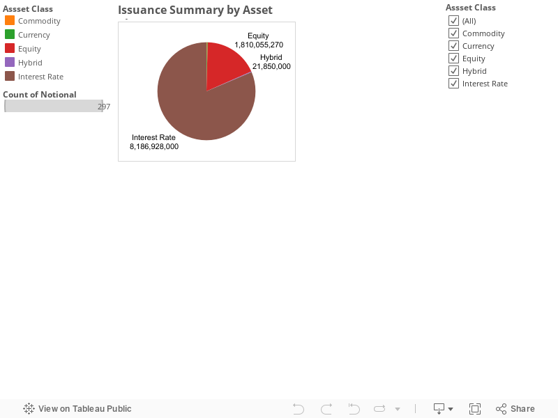
During the week of June 1-13, 2014 structured note issuance has been 10 Bn across various issuers and asset classes. Most of the issuance (1.8 Bn) is driven by Equity Linked notes and 8.1 Bn of the issuance is driven by Interest linked products. There has been some activity in commodity linked issuance this week. For Details of the distribution refer to the chart below. Not surprisingly majority of the structured note issuance is linked to Interest rate linked by few issuers.

This week, structured notes were issued with variety of flavors and interesting themes. Majority of this issuance comprised of Interest Rate related notes Read on for more details.

Learn About Tableau

You can click individual asset classes to see how the underlying issuance has happened within each asset type by underlying and Issuer.

Learn About Tableau

Underlying analysis

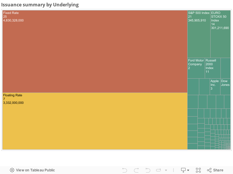
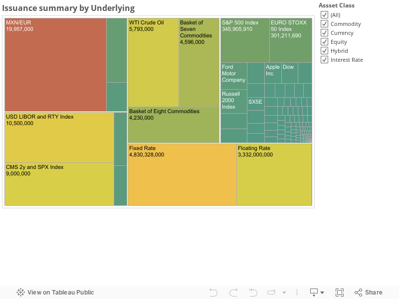
On the Equity linked notes front there has been strong activity. Notes have been created on variety of underlyings. Index related issuance has been significant. This week issuance included notes created on the indices ( S&P 500, Stoxx 50, Russell 2000) and single names ( Face Book, Amazon,Pulte Group, Apple, Yahoo and so on). There has been significant activity around basket linked notes. Looks there is high appetite from institutional investors to conduct their portfolio balancing process.

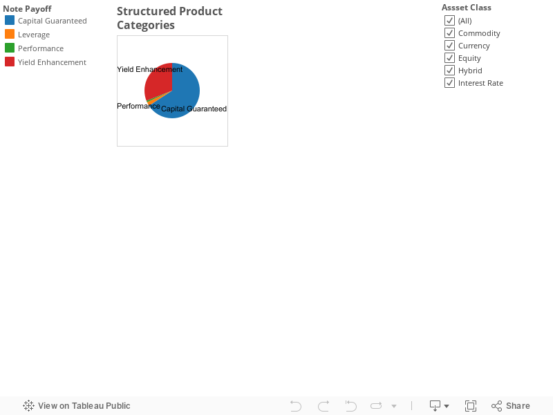
Notable notes this week were tied to SPX Index (144 MM) issued by Credit Suisse. This note belongs to the class of Leveraged Note type. CS created a note 22545F466with a size of 144 MM paying three times Market performance at maturity date (07/31/15) with a coupon capped at 10% and as long as index is above initial level. On the downside this note is exposed to one to one downside underlying performance. Motivation behind participating in this kind of note is to obtain 3 times leverage on the coupon. Another interesting note is on Ford Motor company stock. This looks very high notional for a stock like Ford Mortor company 40434C543 This note belongs to Yield enhancement type and providing a 7% quarterly coupon.

Learn About Tableau

Interest rate linked issuance limited to standard, step up callable notes and Fixed rate notes. Activity has been subdued this week.Citigroup, RBC and AMERICAN HONDA FINANCE CORP are major issuers of these products.

This week we have seen commodity note issuance tied to Commodity Baskets and Crude Oil by Morgan Stanley..

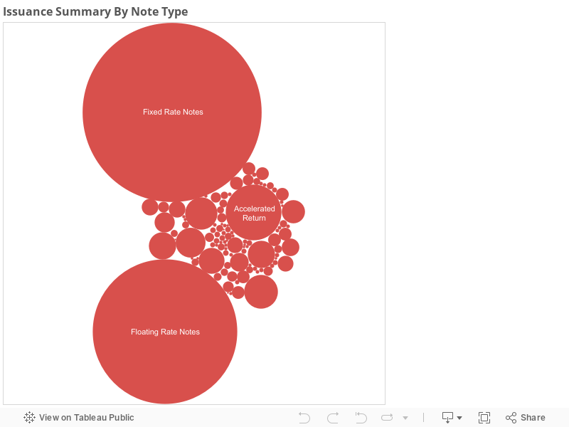
Size of the note types will tell us an indication of what type structures are popular among the investors and where money is flowing. Below chart shows this theme

Learn About Tableau

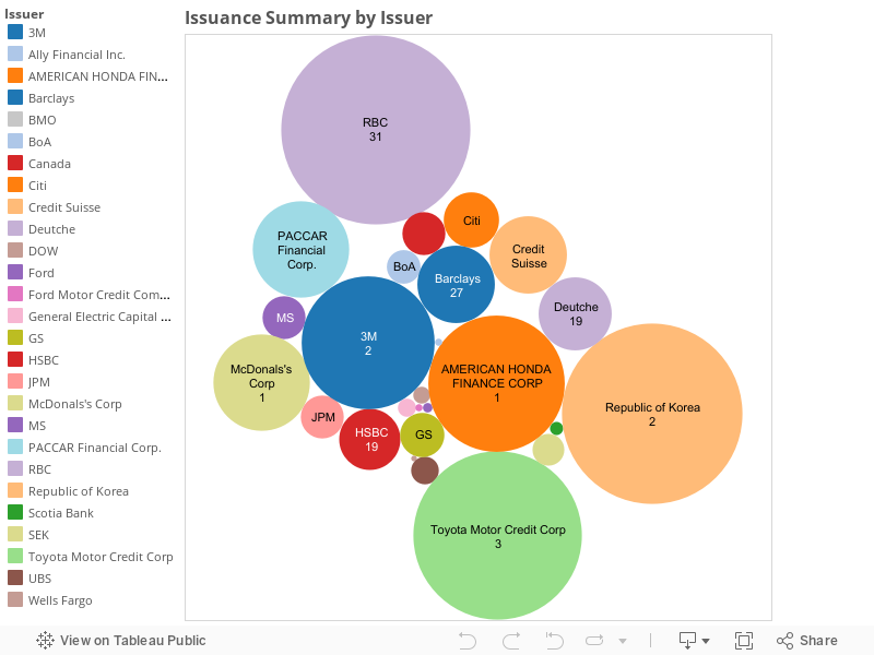
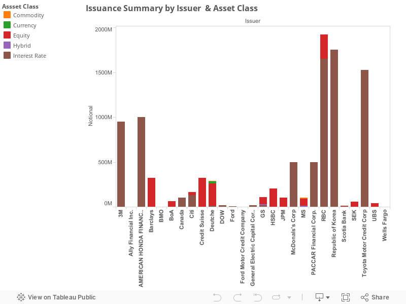
Popular notes have been interest rate linked notes. Now moving on to issuers side and understanding their market penetration or competitor analysis provides some interesting insights. This week UBS, MS, GS and Barclays captured issuance market share.

Learn About Tableau

Market penetration is driven by the issuer depth in each of the asset classes. Every issuer has presence in Equity linked issuance. Goldman is only issuer to produce Currency related issuance. Morgan Stanley and JPM are active players in the Hybrid related issuance.

Learn About Tableau

Learn About Tableau

Learn About Tableau

Learn About Tableau

High charts plus Wordpress

I have struggled 2 days to be able to work with high charts with Wordpress. I guess to save time and effort for someone new who wants to do the same thing, Please follow below steps.


I have read many blogs including forums and I found help from variety of sources and I thanks all of you guys.


 Firstly please read this how someone tried.
 http://forum.highcharts.com/highcharts-usage/is-this-beyond-a-normal-person-t18807/#p76296

 I still was not able to load the high charts. But I have implemented the following steps ( inline with the above link)


 1)Download Highchart software and unzip from http://www.highcharts.com/products/highcharts

2)Now upload all the files with in the js folder into your cpanel. Here one has to be careful in terms of where you are uploading. Locate public_html folder and follow this path to next folder /wp-content/themes/ and then to your themes folder (for instance catch-box) and lastly folder js. It should look like this public_html/wp-content/themes/catch-box/js

 3) Create the directory structure of the Highcharts (js) folder and upload files. (modules, themes, adapter)

 4)Next step is to update Header.php in the folder public_html/wp-content/themes/catch-box

 5) To this file add the following two things

 <script src="http://code.jquery.com/jquery-1.7.1.min.js" type="text/javascript"></script>  
 <br>  
 <script src="&lt;?php bloginfo('template_directory'); ?&gt;/js/highcharts.js" type="text/javascript"></script>"<br />  

 6)Add the following code in a new page

 <html>  
  <head>  
  <title>Rates View - 1</title>  
  <script src="http://ajax.googleapis.com/ajax/libs/jquery/1.8.2/jquery.min.js" type="text/javascript"></script>  
  <script type="text/javascript">  
 $(function () {  
     $('#container').highcharts({  
       chart: {  
         type: 'column'  
       },  
   title: {  
         text: 'Rates - Feb 28 - View - 1',  
         x: -20 //center  
       },  
       subtitle: {  
         text: 'Source: DTCC',  
         x: -20  
       },  
       xAxis: {  
         categories: ['Basis Swaps', 'CapFloors', 'Exotic', 'Fixed Fixed Swaps', 'FRA', 'Inflation Swaps', 'OIS Swaps', 'Swaption', 'Vanilla Swaps', 'X-Ccy-Basis', 'X-Ccy-Fixed-Fixed', 'X-Ccy-Fixed-Float'  
         ]  
       },  
       yAxis: {  
         title: {  
           text: 'Sum of Notional USD'  
         },  
         plotLines: [{  
           value: 0,  
           width: 1,  
           color: '#808080'  
         }]  
       },  
       tooltip: {  
         valueSuffix: 'USD'  
       },  
       legend: {  
         layout: 'horizontal',  
         align: 'right',  
         verticalAlign: 'middle',  
         borderWidth: 0  
       },  
       series: [{  
         name: 'Total',  
         data: [10337207913,28876709079,27143522556,78690127.08,58717429750,4102063542,1.85611E+11,1.21484E+11,3.37014E+11,7116442472,268174806.4,4632368916]  
       }]  
     });  
   });  
  </script>  
  </head>  
  <body>  
 <div id="container" style="height: 400px; margin: 0 auto; min-width: 310px;">  
 </div>  
 </body>  
 </html>  

7) Done.

Pricing an Equity Linked Note - Python-Quantlib

Pricing an Equity Linked Structure Note

By Karthik Misra

This Structure note, created by Barclays, has an aggregates nominal amount of 1.507 million USD. The redemption date for this note is August 1, 2018. Owners of the note will receive interest payments once a month on review days till the redemption date. The interest payment is based on a barrier condition, which requires the linked equity to be above 68.75% of the initial price or 30.09USD. This provides a interest payment of 0.58333. The final payment at maturity note holders will receive 1000USD as long as the equity stays above the barrier of 68.75% of the initial price or 30.09USD. Else if it is below that barrier level whatever the equivalent return should be based on performance.

 Before going into pricing the note itself, discount factors should be created to present value from all the interest payments and principle on maturity. This is done using the ‘USD Yield Curve” building script provided below on March 18, 2014 and modify it slightly on top of the regular input change. The changes can be seen in the bottom where the discount factor is matched with the review dates and saved as a csv.

# Copyright (C) 2014, Khandrika Capital Markets

# This program is distributed in the hope that it will be useful, but WITHOUT
# ANY WARRANTY; without even the implied warranty of MERCHANTABILITY or FITNESS
# FOR A PARTICULAR PURPOSE.  See the license for more details.

from QuantLib import *
import datetime
import numpy as np
import matplotlib
import matplotlib.pyplot as plt
import pandas as pd


# global data
# Here enter the Yield Curve reference Data
calendar = TARGET()
todaysDate = Date(31,March,2014); # should be a weekday
Settings.instance().evaluationDate = todaysDate
settlementDate = Date(2,April,2014); #add 2 days to todaysDate and should be a weekday

# market quotes
# Update deposit Rates ( usual source will be LIBOR Fixings on the Curve Date
deposits = { (1,Weeks): 0.0023,
             (1,Months): 0.0023,
             (3,Months): 0.0023,
             (6,Months): 0.0023}
# Obtain Futures prices from CME traded Euro Dollar Futures ##Data from quantdl
futures = { #Date(19,3,2014): 99.765, #date passed so it was removed
            Date(18,6,2014): 99.75,
            Date(17,9,2014): 99.73,
            Date(17,12,2014): 99.69,
            Date(18,3,2015): 99.605,
            Date(17,6,2015): 99.47,
            Date(16,9,2015): 99.3,
            Date(16,12,2015): 99.085,
            Date(16,3,2016): 99.085,} #Date was added to build curve
# Obtain Swap rates from Traded Swaps on the Curve data
swaps = { (3,Years): 0.0079,
          (4,Years): 0.012,
          (5,Years): 0.0157,
          (6,Years): 0.01865,
          (7,Years): 0.0216,
          (8,Years): 0.0235,
          (9,Years): 0.0254,
          (10,Years): 0.0273,
          (15,Years): 0.0297,
          (20,Years): 0.0316,
          (25,Years): 0.0335,
          (30,Years): 0.0354}

# convert them to Quote objects
for n,unit in deposits.keys():
    deposits[(n,unit)] = SimpleQuote(deposits[(n,unit)])
for d in futures.keys():
    futures[d] = SimpleQuote(futures[d])
for n,unit in swaps.keys():
    swaps[(n,unit)] = SimpleQuote(swaps[(n,unit)])

# build rate helpers

dayCounter = Actual360()
settlementDays = 2
depositHelpers = [ DepositRateHelper(QuoteHandle(deposits[(n,unit)]),
                                     Period(n,unit), settlementDays,
                                     calendar, ModifiedFollowing,
                                     False, dayCounter)
                   for n, unit in [(1,Weeks),(1,Months),(3,Months),
                                   (6,Months)] ]

dayCounter = Actual360()
months = 3
futuresHelpers = [ FuturesRateHelper(QuoteHandle(futures[d]),
                                     d, months,
                                     calendar, ModifiedFollowing,
                                     True, dayCounter,
                                     QuoteHandle(SimpleQuote(0.0)))
                   for d in futures.keys() ]

settlementDays = 2
fixedLegFrequency = Semiannual
fixedLegTenor = Period(6,Months)
fixedLegAdjustment = Unadjusted
fixedLegDayCounter = Thirty360()
floatingLegFrequency = Quarterly
floatingLegTenor = Period(3,Months)
floatingLegAdjustment = ModifiedFollowing
swapHelpers = [ SwapRateHelper(QuoteHandle(swaps[(n,unit)]),
                               Period(n,unit), calendar,
                               fixedLegFrequency, fixedLegAdjustment,
                               fixedLegDayCounter, Euribor3M())
                for n, unit in swaps.keys() ]

# term structure handles

discountTermStructure = RelinkableYieldTermStructureHandle()
forecastTermStructure = RelinkableYieldTermStructureHandle()

# term-structure construction

helpers = depositHelpers[:2] + futuresHelpers + swapHelpers[1:]
depoFuturesSwapCurve = PiecewiseFlatForward(settlementDate, helpers,
                                            Actual360())
rdate=[]
rrate=[]
#replace array with whatever dates you want
c1=[Date(28,4,2014),Date(28,5,2014),Date(26,6,2014),Date(1,8,2014),Date(27,8,2014),Date(26,9,2014),Date(29,10,2014),Date(25,11,2014),Date(29,12,2014),Date(28,1,2015),Date(25,2,2015),Date(27,3,2015),Date(28,4,2015),Date(27,5,2015),Date(26,6,2015),Date(29,7,2015),Date(27,8,2015),Date(28,9,2015),Date(28,10,2015),Date(25,11,2015),Date(29,12,2015),Date(27,1,2016),Date(25,2,2016),Date(29,3,2016),Date(27,4,2016),Date(26,5,2016),Date(28,6,2016),Date(27,7,2016),Date(29,8,2016),Date(28,9,2016),Date(27,10,2016),Date(28,11,2016),Date(28,12,2016),Date(27,1,2017),Date(24,2,2017),Date(29,3,2017),Date(26,4,2017),Date(26,5,2017),Date(28,6,2017),Date(27,7,2017),Date(29,8,2017),Date(27,9,2017),Date(27,10,2017),Date(28,11,2017),Date(27,12,2017),Date(29,1,2018),Date(26,2,2018),Date(27,3,2018),Date(26,4,2018),Date(29,5,2018),Date(27,6,2018),Date(25,7,2018)] 

#print c1
#print depoFuturesSwapCurve.dates()
v=[]
rdate.append(depoFuturesSwapCurve.dates())
for c in c1:
    #print depoFuturesSwapCurve.discount(c)
    v.append([c,depoFuturesSwapCurve.discount(c)])
    rrate.append(depoFuturesSwapCurve.discount(c))

    #pulls the discount factor that correlates with the dates and saves it to csv
v=pd.DataFrame(v)
v.columns=['Date','Df']
v.to_csv('Desktop/lsm_bmy.csv')


Now the note can be priced.  A tweak to the Monte-Carlo Simulation scrip allows this note to be priced.  Specifically simulates the movement of the equity using a standard normal distribution allowing for random interest payments.  Remember to change the csv import location to match the location of the saved csv from above along with all the other normal input changes to match the description on the note. Once the program is done running should see the value of the note as note price. 
	

import pandas as pd
import numpy as np                         # numpy namespace
from timeit import default_timer as timer  # for timing
from matplotlib import pyplot              # for plotting
import math

def step_numpy(dt, prices, c0, c1, noises):
    return prices * np.exp(c0 * dt + c1 * noises)

def pricer(paths, dt,Dividend, interest, volatility):
    c0 = interest -  Dividend- 0.5 * volatility ** 2
    c1 = volatility * np.sqrt(dt)

    for j in xrange(1, paths.shape[1]):   # for each time step
        prices = paths[:, j - 1]          # last prices
        # gaussian noises for simulation
        noises = np.random.normal(0., 1., prices.size)
        # simulate
        paths[:, j] = step_numpy(dt, prices, c0, c1, noises)



StockPrice=53.15           #StockPrice 
StrikePrice=53.15          #StrikePrice 
Volatility=.25493          #Volatility 
InterestRate=.012          #InterestRate
Maturity=4.58333           #Maturity 
Dividend=.005016           #Dividend 
CP=-1                      #CP = 1/-1 for call/put
ot=1                       #ot = 1/2/3 for vinilla/asian/barrier
NumPath=100000             #NumPath = number of runs
NumStep=52                 #NumStep = number of steps in each run should be the number of payments
#MAX_PATH_IN_PLOT=

    #Preparation
paths = np.zeros((NumPath, NumStep + 1), order='F')
paths[:, 0] = StockPrice
DT = Maturity / NumStep
df = np.exp(-InterestRate * DT)

    #Simulation
ts = timer()
pricer(paths, DT,Dividend, InterestRate, Volatility)
te = timer()
elapsed = te - ts

ST = paths[:, -1]

    #Creates coupon payment for simulation streams adjust as needed
h1=np.where(paths[:,:]>=30.09,0.58333,0)  #adjust as needed


h= np.maximum(CP*(paths - StrikePrice), 0)
V = np.zeros_like(h)  # value matrix
V[:,-1] = h[:,-1]

    # Valuation by LSM
#for t in range(NumStep - 1, 0, -1):
#    rg = np.polyfit(paths[:,t], V[:, t+1] * df, 5)  # regression
#    C = np.polyval(rg, paths[:,t])  # evaluation of regression
#    V[:,t] = np.where(h[:,t] > C, h[:,t],V[:, t+1] * df)  # exercise decision/optimization



#V0 = np.sum(V[:, 1] * df) / NumStep  # LSM estimator
#V1= np.average(V[:, 1] * df) / NumStep
#if ot==1:
#    PaidOff = np.maximum(CP*(paths[:, -1] - StrikePrice), 0)
#elif ot==2:
#    PaidOff = np.maximum(CP*(np.average(paths[:,]) - StrikePrice), 0)
#    
#elif ot==3:
#    PaidOff = np.maximum(CP*((paths[:, -1]>=BarrierLevel) - StrikePrice), 0)
#elif ot==4:
#    PaidOff = np.maximum(CP*((paths[:, -1]<=BarrierLevel) - StrikePrice), 0)
    

    #Accounts for payment on maturity adjust as needed
h1[:,-1]=np.where(paths[:,-1]>=30.09,100.0,(100.0*(paths[:,-1]/43.76)))  #adjust as needed

    #Creates an vector to discount
q1=np.zeros_like(h1)

    #imports discount factor from csv as an array
#df1=np.genfromtxt('Desktop/DF_BMY.csv', delimiter=',')
df=pd.read_csv('Desktop/lsm_bmy.csv')
df=df.ix[:,'Df']
df1=[]
df1[:]=df

    #discounts all payments
for x in range(0,NumStep):
    q1[:,x]=h1[:,x]*df1[x]
    #q1[:,x]=h1[:,x]/((1+InterestRate)**x)
q2=np.sum(q1[:,], axis=1)
gc=np.average(q2)

    #discounts final payment on maturity
q3=h1[:,-1]*df1[-1]    
g=np.average(q3)



print 'Result'
fmt = '%20s: %s'


print fmt % ('principal', g)
print fmt % ('coupon cash flows', gc)
print fmt % ('Note price', (g+gc))
print 'Performance'
NumCompute = NumPath * NumStep
print fmt % ('Mstep/second', '%.2f' % (NumCompute / elapsed / 1e6))
print fmt % ('time elapsed', '%.3fs' % (te - ts))

 	A run of this program, with a 100000 simulations, provided a result where the principle was 85.1438664683. The coupon cash flows is 27.140993899 with the note price being $113.284860367.

Role of Derivatives in Global Economy - Study by CME and Milken Group

Derivatives – are good for economy argues Apanard (Penny) Prabha, Keith Savard  and Heather Wickramarachi in a study published by Milken institute.  In this study have analyzed and quantified derivatives impact and concluded,

http://www.cmegroup.com/education/growth-through-risk-management.html

“KEY FINDINGS

»≫Banks’ use of derivatives, by permitting greater extension of credit to the private sector, increased U.S. quarterly real GDP by about $2.7 billion each quarter from Q1 2003 to Q3 2012.

»≫Derivatives use by non-financial firms increased U.S. quarterly real GDP by about $1 billion during the same period by improving their ability to undertake capital investments.

»≫Combined, derivatives expanded U.S. real GDP by about $3.7 billion each quarter. The total increase in economic activity was 1.1 percent ($149.5 billion) between 2003 and 2012.

»≫By the end of 2012, employment had been boosted by 530,400 (0.6 percent) and industrial production 2.1 percent.”

Derivatives are termed as Financial WMD by famed investor Warren Buffet. In the wake of great financial crisis of 2008 regulators have focused on bringing transparency to Derivatives trading blaming some of these products do not provide any value to the society. This study first of its kind in terms of not only putting together case studies on how Air line carriers hedge their oil cost by using Oil based derivatives, Food processor hedging his production costs by utilizing grain based contracts and most importantly how banks are able to intermediate loans by managing their interest rate risk but also building a quantitative model to back their analysis.

“WHY USE DERIVATIVES?

Investors generally use derivatives for three purposes: risk management, price discovery, and reduction of transaction costs. In a traditional banking model, a maturity mismatch between assets and liabilities subjects banks to interest rate risk. Derivatives mitigate this risk, which often contributes to capital adequacy, profitability, and lowering the probability of bank failure. In addition, banks make markets in derivatives to meet the risk management needs of financial and non-financial firm customers. In the process, they generate fees and other revenue from this trading as well as lower their cost of funding.

Derivatives Help Price discovery

The information that can be extracted from derivatives, such as price discovery, is another important benefit. In “complete” markets (when agents can buy insurance contracts to protect against any future state of the world), trading on derivative exchanges should reveal no new information to market participants. However, the lack of completeness means that informed traders could prefer to own futures or options in lieu of the underlying assets, and this might reveal new information about price. Most studies done on developed nations show that the futures market leads the spot market and therefore serves as the focal point for price discovery.”

I totally agree on all three points that derivatives, are helping in risk management, price discovery and reduction of transaction costs. For instance, when we consider housing market where a typical home buyer goes out to take a 30y fixed rate loan from his bank. Bank hedges this loan on its books with various interest rate derivatives (swaps) to risk manage the interest rate risk. In doing so they transact swaps leading to activity in the swap market and price discovery and leading to better rates to the home buyer.

Authors have chronicled the history of Derivatives in terms of when they started to current day regulatory environment. Growth in the trading volumes of derivative products clearly coincided with increase on global trade and rise in both bond and Equity markets.

“Given the expansion of international trade and financial activities, participants are likely to face increasing risks, and derivatives markets are expected to contribute to economic development by making these risks manageable.”

Interesting fact here to see how big Derivative markets are when compared to global GDP.

After looking at the Trading volumes focus has moved to how this growth has benefited overall economy within the framework of Risk, Price and Cost factors.

Banks use derivatives predominantly to manage the risk arising due to their banking and trading operations. Below chart shows how banks have started increasing using the derivatives on their books. Most of this derivative activity is concentrated in the hands of few large banks. As OCC’s quarterly report confirms, four big banks, JP morgan, Bank of America, Citi bank and Goldman Sachs have had lion’s share of the market.

For nonfinancial Firms Derivative have been serving purely for hedging purposes.

Below chart shows how derivatives have saved some of these firms big money.

This chart provides details of how various users of the Derivative market come together for their needs and consequently affecting the economy. Interestingly, nonfinancial firms are able to increase their firm value by using these products to hedge cash flow volatility.

Banks that use derivatives to manage their operations are able to increase their loans. Below another chart that shows this positive relationship between loan growth and Derivatives usage.

Authors have studied above relationships and confirmed usage of Derivatives is benefiting the Real GDP and increase in employment.